Building a new model library
For most new applications, a model will need to be constructed. This will include adjustable parameters which Fabber will then fit.
The example shown below is included in the examples subdirectory of
the Fabber source code. This provides an easy template to implement a
new model.
We will assume only some basic knowledge of C++ for this example.
A simple example
To create a new Fabber model it is necessary to create an instance of
the class FwdModel. As an example, we will create a model which fits the
data to sum of exponential functions, each with an amplitude and decay rate.
Note
The source code and Makefile file for this example are in the
Fabber source code, in the examples subdirectory. We will assume you
have this to hand as we go through the process!
First we will create the interface fwdmodel_exp.h file which shows the methods we
will need to implement:
// fwdmodel_exp.h - A simple exponential sum model
#pragma once
#include "fabber_core/fwdmodel.h"
#include "newmat.h"
#include <string>
#include <vector>
class ExpFwdModel : public FwdModel {
public:
static FwdModel* NewInstance();
ExpFwdModel()
: m_num(1), m_dt(1.0)
{
}
std::string ModelVersion() const;
std::string GetDescription() const;
void GetOptions(std::vector<OptionSpec> &opts) const;
void Initialize(FabberRunData &args);
void EvaluateModel(const NEWMAT::ColumnVector ¶ms,
NEWMAT::ColumnVector &result,
const std::string &key="") const;
protected:
void GetParameterDefaults(std::vector<Parameter> ¶ms) const;
private:
int m_num;
double m_dt;
static FactoryRegistration<FwdModelFactory, ExpFwdModel> registration;
};
We have not made our methods virtual, so nobody will be able to create a subclass of our model. If we wanted this to be the case all the non-static methods would need to be virtual, and we would need to add a virtual destructor. This is sometimes useful when you want to create variations on a basic model (for example we have a variety of DCE models all inheriting from a common base class).
Most of the code above is completely generic to any model. The only parts which are specific to our exp-function model are:
- The name
ExpFwdModel- The private variables
m_num(the number of exponentials in our sum) andm_dt(the time between data points).
We will now implement these methods one by one. Many of them are
straightforward. We start our implementation file fwdmodel_exp.cc as follows:
//  fwdmodel_exp.cc - Implements a simple exp curve fitting model
#include "fwdmodel_exp.h"

#include <fabber_core/fwdmodel.h>

#include <math.h>

using namespace std;
using namespace NEWMAT;
This just declares some standard headers we will use. If you prefer to fully qualify your
namespaces you can leave out the using namespace lines.
We need to implement a couple of methods to ensure that our model is visible to the Fabber system:
FactoryRegistration<FwdModelFactory, ExpFwdModel> ExpFwdModel::registration("exp");

FwdModel* ExpFwdModel::NewInstance()
{
    return new ExpFwdModel();
}
The first line here registers our model so that it is known to Fabber by
the name exp The second line is a Factory method used so that
Fabber can create a new instance of our model when its name appears on
the command line:
string ExpFwdModel::ModelVersion() const
{
    return "1.0";
}

string ExpFwdModel::GetDescription() const
{
    return "Example model of a sum of exponentials";
}
We’ve given our model a version number, if we update it at some later stage we should change the number returned so anybody using the model will know it has changed and what version they have. There’s also a brief description which fabber will return when the user requests help on the model:
static OptionSpec OPTIONS[] = {
    { "dt", OPT_FLOAT, "Time separation between samples", OPT_REQ, "" },
    { "num-exps", OPT_INT, "Number of independent exponentials in sum", OPT_NONREQ, "1" },
    { "" }
};

void ExpFwdModel::GetOptions(vector<OptionSpec> &opts) const
{
    for (int i = 0; OPTIONS[i].name != ""; i++)
    {
        opts.push_back(OPTIONS[i]);
    }
}
This is the suggested way to declare the options that your model can
take - in this case the user can choose how many exponentials to include in the sum
and what the time resolution in the data is. Each option is listed in the OPTIONS array which
ends with an empty option (important!).
An option is described by:
- It’s name which generally should not include underscores (hyphen is preferred as in this case). The name translates into a command line option e.g.
--num-exps.
- An option type. Possibilities are:
OPT_BOOLfor a Yes/No option which is considered ‘off’ unless it is specifiedOPT_FLOATfor a decimal numberOPT_INTfor a whole number (integer)OPT_STRfor textOPT_MATRIXfor a small matrix (specified by giving the filename of a text file which contains the matrix data in tab-separated form)OPT_IMAGEfor a 3D image specified as a Nifti fileOPT_TIMESERIESfor a 4D image specified as a Nifti fileOPT_FILEfor a generic filename- A brief description of the option. This will be displayed when
--helpis requested for the modelOPT_NONREQif the option is not mandatory (does not need to be specified) orOPT_REQif the option must be provided by the user.- An indication of the default value. This value is not used to initialize anything but is shown in
--helpto explain to the user what the default is if the option is not given. So it can contain any text (e.g."0.7 for PASL, 1.3 for pCASL". You should not specify a default for a mandatory option (OPT_REQ)
In this case we have made the time resolution option mandatory because we have no reasonable way to guess this, but the number of exponentials defaults to 1.
This option system is a little cumbersome when there is only a couple of options, but if you have many it will make it clear to see what they are. Most real models will have many configuration options, for example an ASL model will need to know details of the sequence such as the TIs/PLDs, the bolus duration, the labelling method, number of repeats, etc…
Options specified by the user are captured in the FabberRunData
object which we use to set the variables in our model class
in the Initialize method. Initialize is called before the model
will be used. Its purpose is to allow the model to set up any internal
variables based on the user-supplied options. Here we capture the
time resolution option and the number of exponentials - note that
the latter has a default value:
void ExpFwdModel::Initialize(FabberRunData& rundata)
{
    m_dt = rundata.GetDouble("dt");
    m_num = rundata.GetIntDefault("num-exps", 1);
}
The lack of a default value for dt means that an exception will be thrown
if this option is not specified.
We use the term Options to distinguish user-specified or default model configuration from Parameters which are the variables of the model inferred by the Fabber process. Next we need to specify what parameters our model includes:
void ExpFwdModel::GetParameterDefaults(std::vector<Parameter> ¶ms) const
{
params.clear();
int p=0;
for (int i=0; i<m_num; i++) {
params.push_back(Parameter(p++, "amp" + stringify(i+1), DistParams(1, 100), DistParams(1, 100), PRIOR_NORMAL, TRANSFORM_LOG()));
params.push_back(Parameter(p++, "r" + stringify(i+1), DistParams(1, 100), DistParams(1, 100), PRIOR_NORMAL, TRANSFORM_LOG()));
}
}
GetParameterDefaults is quite important. It declares the parameters our
model takes, and their prior and initial posterior distributions. It is always
called after Initialize so you can use whatever options you have set up to
decide what parameters to include.
The code above declares two parameters named amp<n> and r<n> for each exponential
in the sum, where <n> is 1, 2, … As well as a name, each parameter has two DistParams
instances defining the prior and initial posterior distribution for the parameter.
DistParams take two parameters - a mean and a variance. At this
point we will diverge slightly to explain what these mean.
Priors and Posteriors
Priors are central to Bayesian inference, and describe the extent of our belief about a parameter’s value before we have seen any data.
For example if a parameter represents the \(T_1\) value of grey matter in the brain there is a well known range of plausible values. By declaring a suitable prior we ensure that probabilities are calculated correctly and unlikely values of the parameter are avoided unless the data very strongly supports this.
In our case we have no real prior information, so we are using an uninformative prior.
This has a large variance so the model has a lot of freedom in fitting the parameters and
will try to get as close to matching the data as it can. This is reflected in the high
variance we are using (1e6). For the mean values, a and b are multiplicative so
it makes sense to give them defaults of 1 wherease c and d are additive so
prior means of 0 seems more appropriate.
The second DistParams instance represents the initial posterior. This is the starting
point for the optimisation as it tries to find the best values for each parameter. Since the
optimization process should iterate to the correct posterior, this may not matter too much
and can often be set to be identical to the prior.
When using a non-informative prior, however, it may be better to give the initial posterior a more restrictive (lower) variance to avoid numerical instability. We have done that here, using 100 for the initial posterior variance.
There is rarely a good reason to set the initial posterior to have a different mean to the prior globally. However it is possible to adjust the initial posterior on a per-voxel basis using the actual voxel data. We will not do that here, but it can be useful when fitting, for example, a constant offset, where we can tell the optimisation to start with a value that is the mean of the data. This may help avoid instability and local minima.
In general it is against the spirit of the Bayesian approach to modify the priors on the basis of the data, and we don’t provide a method for doing thsi. It is possible for the user to modify the priors on a global basis but this is not encouraged and in general a model should try to provide good priors that will not need modification.
We now go back to our code where we finally reach the point where we calculate the output of our model:
void ExpFwdModel::EvaluateModel(const NEWMAT::ColumnVector ¶ms,
NEWMAT::ColumnVector &result,
const std::string &key) const
{
result.ReSize(data.Nrows());
result = 0;
for (int i=0; i<m_num; i++) {
double amp = params(2*i+1);
double r = params(2*i+2);
for (int i=0; i < data.Nrows(); i++)
{
double t = double(i) * m_dt;
double val = amp * exp(-r * t);
result(i+1) += val;
}
}
}
We are given a list of parameter values (params)
and need to produce a time series of predicted data values (result). We
do this by looping over the parameters and adding the result of each
exponential to the output result.
The additional argument key is not required in this case. It is used
to allow a model to evaluate ‘alternative’ outputs such as an interim
residual or AIF curve. These are not used in the fitting process but can
be written out using the --save-model-extras option.
Note that the variable data is available
at this point and contains the current voxel’s time series. We are using
it here to determine how many time points to generate.
Making the example into an executable
We need one more file to build our new model library into it’s own Fabber executable.
This is called fabber_main.cc and it is very simple:
#include "fabber_core/fabber_core.h"

int main(int argc, char **argv)
{
    return execute(argc, argv);
}
Any number of models can be included in a library. The resulting executable
will contain all the new models we define alongside the default generic
models linear and poly.
Note
It is also possible to build Fabber models into a shared library
which can be loaded dynamically by any Fabber executable. We will
not do that in this example but if you’re interested look at the
additional source files exp_models.cc and exp_models.h
for details.
Building an executable with our new model
The example template comes with a Makefile which can be used
to build the model library using the FSL build system. First you
need to set up an FSL build environment as described in Building Fabber.
Then to build and install our new model library we can just do:
make install
This creates an executable fabber_exp which installs into
$FSLDEVDIR/bin. This executable contains the built-in
generic models and also our new model - you can see this by running:
fabber_exp --listmodels
fabber_exp --help --model=exp
Testing the model - single exponential
A Python interface to Fabber is available which includes a simple
self-test framework for models. To use this you will need to get
the pyfab package - see pyfab.readthedocs.io for more information
on installing this package.
Once installed a simple test script for this model might look like this
(this script is included in the example with the name test_single.py:
#!/bin/env python
import sys
import traceback

from fabber import self_test, FabberException

save = "--save" in sys.argv
try:
    rundata= {
        "model" : "exp",      # Exponential model
        "num-exps" : 1,            # Single exponential function
        "dt" : 0.02,          # With 100 time points time values will range from 0 to 2
    }
    params = {
        "amp1" : [1, 0.5],    # Amplitude
        "r1" : [1.0, 0.8],    # Decay rate
    }
    test_config = {
        "nt" : 100,           # Number of time points
        "noise" : 0.1,        # Amplitude of Gaussian noise to add to simulated data
        "patchsize" : 20,     # Each patch is 20 voxels along each dimension
    }
    result, log = self_test("exp", rundata, params, save_input=save, save_output=save, invert=True, **test_config)
except FabberException, e:
    print e.log
    traceback.print_exc()
except:
    traceback.print_exc()
The test script generates a test Nifti image containing ‘patches’ of data chequerboard style, each of which corresponds to a combination of true parameter values. As Fabber is designed to work on 3D timeseries data you can only vary three model parameters in each test - others must have fixed values.
The test data is generated both ‘clean’ and with added Gaussian noise of specified amplitude. The model is then run on the noisy data to determine how closely the true parameter values can be recovered. In this case we get the following output:
python test_single.py --save

Running self test for model exp
Saving test data to Nifti file: test_data_exp
Saving clean data to Nifti file: test_data_exp_clean
Inverting test data - running Fabber: 100%

Parameter: amp1
Input 1.000000 -> 0.999701 Output
Input 0.500000 -> 0.500674 Output
Parameter: r1
Input 1.000000 -> 1.000728 Output
Input 0.800000 -> 0.801230 Output
Noise: Input 0.100000 -> 0.099521 Output
For each parameter, the input (ground truth) value is given and also the mean inferred value across the patch. In this case it has recovered the parameters pretty well on average. An example plot of a single voxel might look like this:
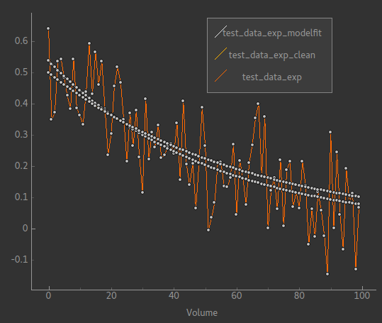
The orange line is the noisy data it’s trying to fit while the two smooth lines represent the ‘true’ data and the model fit. In fact for this example typically the model fit is much closer to the true data - we have chosen this voxel as an example so it is possible to see them separately!
Testing the model - bi-exponential
Fitting to a single exponential is not too challenging - here we will test fitting to a bi-exponential where there are two different decay rates. We will find that we need to improve the model to get a better fit.
First we can modify the test script to test a bi-exponential
(test_biexp.py in examples):
#!/bin/env python

import sys
import traceback

from fabber import self_test, FabberException

save = "--save" in sys.argv
try:
    rundata= {
        "model" : "exp",
        "num-exps" : 2,
        "dt" : 0.02,
        "max-iterations" : 50,
    }
    params = {
        "amp1" : [1, 0.5],    # Amplitude first exponential
        "amp2" : 0.5,         # Amplitude second exponential
        "r1" : [1.0, 0.8],    # Decay rate of first exponential
        "r2" : 6.0,           # Decay rate of second exponential
    }
    test_config = {
        "nt" : 100,           # Number of time points
        "noise" : 0.1,        # Amplitude of Gaussian noise to add to simulated data
        "patchsize" : 20,     # Each patch is 20 voxels along each dimension
    }
    result, log = self_test("exp", rundata, params, save_input=save, save_output=save, invert=True, **test_config)
except FabberException, e:
    print e.log
    traceback.print_exc()
except:
    traceback.print_exc()
This is similar to the last test but we have set num-exps to 2 and added
parameters for a fixed second exponential curve with a faster decay rate.
If we run this we get output something like this:
python test_biexp.py --save
Running self test for model exp
Saving test data to Nifti file: test_data_exp
Saving clean data to Nifti file: test_data_exp_clean
Inverting test data - running Fabber: 100%

Parameter: amp1
Input 1.000000 -> 0.633822 Output
Input 0.500000 -> 0.309912 Output
Parameter: r1
Input 1.000000 -> 19693700210770313216.000000 Output
Input 0.800000 -> -324689116576874496.000000 Output
Noise: Input 0.100000 -> 0.150277 Output
This isn’t looking too encouraging. If we examine the model fit against the data we find that actually most voxels have fitted quite well:
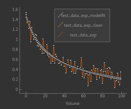
However a few voxels have ended up with very unrealistic parameter values. This kind of behaviour is a risk with model fitting - in trying to find the best solution the inference can end up finding a local minimum which is a long way from the true minimum.
We will show two additions we can make to our model to improve this behaviour.
Initialising the posterior
The initial posterior is a ‘first guess’ at the parameter values
and can be based on the data. Fabber models can use their knowledge
of the model to make a better guess by overriding the InitVoxelPosterior
method. We firstly add this method to fwdmodel_exp.h:
void InitVoxelPosterior(MVNDist &posterior) const;
Now we implement it in fwdmodel_exp.cc:
void ExpFwdModel::InitVoxelPosterior(MVNDist &posterior) const
{
    double data_max = data.Maximum();

    for (int i=0; i<m_num; i++) {
        posterior.means(2*i+1) = data_max / (m_num + i);
    }
}
Our implementation only affects the amplitude and sets an initial guess so that the sum of all our exponentials is close to the maximum data value. Note that we make the posterior means different for each exponential - this helps break the symmetry of the inference problem.
Parameter transformations
A major reason for the failure of some voxels to fit is that
the decay rate in particular could become negative, generating
an exponential increase curve which may be so far away from the
data that it does not successfully converge back to the correct
value. In many models we want to restrict parameters to positive
values to prevent this sort of unphysical solution. One way to
do this is to use a log-transform of the parameter (i.e. assuming
the parameter takes a log-normal distribution rather than a
standard Gaussian). We can do this by modifying GetParameterDefaults
as follows:
void ExpFwdModel::GetParameterDefaults(std::vector<Parameter> ¶ms) const
{
params.clear();
int p=0;
for (int i=0; i<m_num; i++) {
params.push_back(Parameter(p++, "amp" + stringify(i+1), DistParams(1, 100), DistParams(1, 100), PRIOR_NORMAL, TRANSFORM_LOG()));
params.push_back(Parameter(p++, "r" + stringify(i+1), DistParams(1, 100), DistParams(1, 100), PRIOR_NORMAL, TRANSFORM_LOG()));
}
}
(we also need to add #include <fabber_core/priors.h> at the top of fwdmodel_exp.cc.
With these changes we still retain some bad fitting voxels but fewer than previously. The output of the test script is now:
python test_biexp.py --saveike this::
Running self test for model exp
Saving test data to Nifti file: test_data_exp
Saving clean data to Nifti file: test_data_exp_clean
Inverting test data - running Fabber: 100%

Parameter: amp1
Input 1.000000 -> 0.714108 Output
Input 0.500000 -> 0.498471 Output
Parameter: r1
Input 1.000000 -> 4.898833 Output
Input 0.800000 -> 4.674414 Output
Noise: Input 0.100000 -> 0.099399 Output
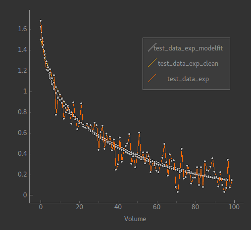
So we clearly have a reduction in the number of extreme values. In this case we can’t actually trust the
self-test output because sometimes the inference ‘swaps’ the exponentials around making
amp1 = amp2 and r1 = r2. But viewing the model fit
visually shows sensible fitting in the overwhelming majority of voxels:
Changing the example to your own model
To summarize, these are the main steps you’ll need to take to change this example into your own new model:
- Edit the
Makefileto change references toexpandExpto the name of your model - Rename source files, e.g.
fwdmodel_exp.cc->fwdmodel_<mymodel>.cc - Add your model options to the options list in the
.ccfile - Add any model-specific private variables in the
.hfile - Implement the
Initialize,GetParameterDefaults,Evaluatemethods for your model. - If required, implement
InitVoxelPosterior